Project Final Report
Contribution Table
| Task | Member |
|---|---|
| Continue CNN | Ray |
| SVM | Aiden |
| Add to Report, Presentation, and Video | All |
| Github Organization | Charlie |
Background
Deaf and hard-of-hearing people face issues with communication every day, relying only on sign language. However, with barely any education in schools, people without these disabilities often fail to interpret sign language. This issue is very common for Bengali Sign Language (BdSL) users due to the lack of research in the area and the number of BdSL interpreters. We aim to mitigate this problem. Our system would rely on images of bare hands in varied positions, providing a natural experience for users.
Problem Definition
Beginners may find it challenging to differentiate between the Bengali sign language alphabet’s symbolic variations. A program that generates a real-time analysis of hand movement will help consumers to increase the efficiency and accuracy of their learning process while giving them valuable input to improve the experience. Additionally, we believe that people who do not understand the Bengali sign language will be able to converse with the users of this language easily. We aim to build a computer vision-based system for the automatic recognition of Bengali sign languages to mitigate this problem.
Data Collection
Bengali Sign Language Dataset. (2020, March 8). Kaggle. Retrieved October 3, 2022, from https://www.kaggle.com/datasets/muntakimrafi/bengali-sign-language-dataset
The data was published on Kaggle with a paper in IEEE. The research was sponsored by the Bangladesh University of Engineering and Technology in collaboration with the National Federation of the Deaf (Bangladesh).
We used the dataset directly in a Kaggle notebook. We also downloaded it and uploaded it to GitHub. The dataset contains 12,581 different hand images belonging 38 BdSL signs.
Preprocessing Methods
Background and Shadow Removal
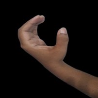
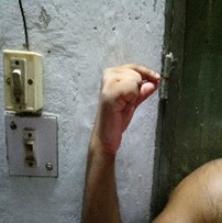
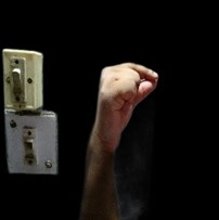
Most of the images we take in real life contain various backgrounds and shadows. To reflect this condition, our data set contains various backgrounds and shadows. For this reason, to increase the accuracy of data set analysis, it is essential for us to remove the background and shadows. Background and shadow removal removes any kind of objects, lighting, and shadows that we do not need. To remove the background and shadows, we used the rembg tool. Unlike other background and shadow removal tools that use simple mathematical calculations, the rembg tool produces much more accurate results by using a neural network-based U2Net. However, the rembg tool does not output 100% accuracy. If you look at the images below, you can see that the image 1 has the background and shadows removed well, but the image 2 has a little background left. However, the result of the rembg tool does not change that it produces much more accurate results than the results of other background and shadow removal tools. As a result of the inspection, the rembg tool completely removed the background and shadows of more than 98% of the images.

Brightness and Contrast Enhancer
To train our model properly based on the dataset, we increased the brightness of the images and enhanced contrasts for the same. This allows for the model to correctly identify and differentiate the different alphabets. We used the Python Imaging Library to perform these tasks on our dataset.
Data Augmentation
To increase the size of our dataset and reduce the possibility for overfitting, we add Keras preprocessing layers that randomly rotate and flip images horizontally/vertically. We believe adding random rotation and flipping makes sense in the real world since if we were to deploy this computer vision model to read Bengali Sign Language, it is possible that the image captured by the camera could be from different angles and sometimes even upside down.
Models
We will use two model types, convolutional neural network (CNN) and support vector machine (SVM).
Convolutional Neural Network
For CNN, we used famous architectures such as AlexNet (Krizhevsky et al., 2017), ResNet50 (He et al., 2016), and MobileNetV2 (Sandler et al., 2018). We use Tensorflow Keras to train these CNN models. For AlexNet, we trained the model from scratch using SGD optimizer and Adam optimizer. For ResNet50 and MobileNetV2, we trained both from scratch and with transfer learning. We only used Adam optimizer for ResNet50 and MobileNetV2. For transfer learning, we pre-loaded the model with weight from imagenet, froze them, and removed the final layer and added a custom fully connected layer for our classification task prediction.
Support Vector Machine
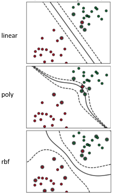
SVM implementation consists of (1) svc declaration, (2) svc fitting, and (3) svc prediction. The svc declaration involves a kernel and gamma that determine the method and degree of svc fitting. The kernels that determine the method of svc fitting are mainly linear, poly, and RBF. Linear makes the svc fitting the simplest and takes little time, while poly and RBF make the svc fitting more flexibly and accurately but take a relatively long time. Reference images for linear, poly, and RBF are as follows. For SVM, we used linear as the method of svc fitting.
Results & Discussion
Convolutional Neural Network
To evaluate the performance of the models, we measured their accuracy and loss. We also measured their average f1 and roc auc score across all classes, which can be calculated by passing in macro as argument to the average parameter in the associated sklearn.metrics. Additionally, we looked at the confusion matrix to inspect the classification result for each class in more detail.
First, to compare different data preprocessing techniques, we trained several models from scratch using the AlexNet architecture with different data preprocessing techniques. We used SGD optimizer (learning rate 0.001, momentum 0.9) and stopped training after no improvement in training loss for 10 epochs and restored the weights from the epoch with minimal loss (use tf.keras.callbacks.EarlyStopping).
The following table compares the results of training with different data preprocessing techniques and data augmentation settings.
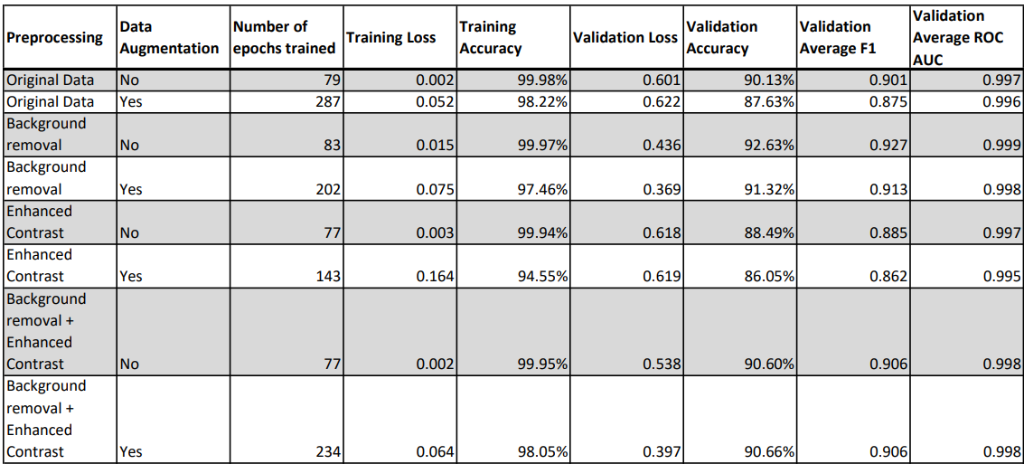
Comparing different data preprocessing techniques, background removal seems to be the most effective in terms of improving testing accuracy while enhancing contrasts doesn’t seem to help much and even has an adverse effect. After introducing data augmentation to combat overfitting, we observed that the training loss increased, and the testing loss decreased in cases where we applied background removal. However, testing loss increased in other cases. Overall, applying background removal plus data augmentation seems to give us the best result. And we will use this setting to train future models.
Next, we new models using AlexNet, ResNet50, and MobileNetV2 as described in the methods section. For all models, we used Adam optimizer with learning rate 0.0001. This time, we stopped training after no improvement in training loss for 7 epochs and restored the weights from the epoch with minimal loss.
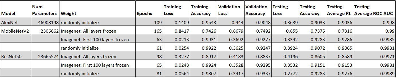
Overall, our result shows that all of them are able to achieve 90% accuracy or higher when training from scratch or with transfer learning and froze the first 100 layers. Specifically, ResNet50 and MobileNetV2 are able to achieve 92.8% testing accuracy, which is a little bit higher than the results from Rafi et al. (2019), where they achieved a test accuracy of 89.6% using an architecture similar to VGG19. It is worth noticing that MobileNetV2, a much smaller model with much less parameters compared to AlexNet or ResNet50, is still able to achieve 92.8% accuracy, which suggests that training a model that can be deployed on mobile devices is possible.
Additionally, based on the result, transferring learning did not produce better models in the end. At first we froze all layers in the base model, and the resulting models were performing poorly. Then, we froze only the first 100 layers and left the rest layers to be trainable, and the results improved significantly.
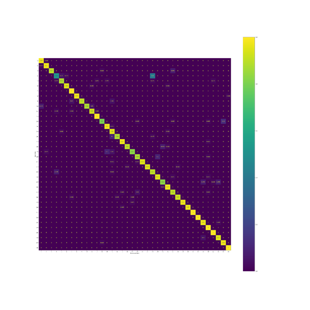
The following is the confusion matrix from the ResNet50 model trained from scratch:
Support Vector Machine
While CNN models showed high accuracy, SVM showed low accuracy of ~30%.
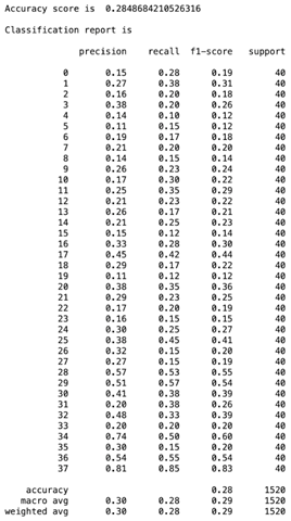
Analysis of the results revealed that there are two reasons for the low accuracy. First, SVM is not very effective when there are many categories. SVM puts the objects on a plane and draws lines to separate the objects. Therefore, the more categories exist, the more difficult it is to accurately separate the objects by drawing lines. The Bengali Sign Language we used for this project has 38 categories. Second, the method of svc fitting we used was linear. As you saw reference images for linear, poly, and RBF above, linear as a svc fitting method is very likely to create an inflexible separation. However, through this result, we thought that poly and RBF, which draw curves, would give better results. Therefore, we decided to not stop at this point. As an extension of this project, we are going to check whether poly and RBF as svc fitting methods would give better results.
References
He, K., Zhang, X., Ren, S., & Sun, J. (2016). Deep residual learning for image recognition. In Proceedings of the IEEE conference on computer vision and pattern recognition (pp. 770-778). http://openaccess.thecvf.com/content_cvpr_2016/html/He_Deep_Residual_Learning_CVPR_2016_paper.html
Krizhevsky, A., Sutskever, I., & Hinton, G. E. (2017). Imagenet classification with deep convolutional neural networks. Communications of the ACM, 60(6), 84-90. https://dl.acm.org/doi/abs/10.1145/3065386
Rafi, A. M., Nawal, N., Bayev, N. S. N., Nima, L., Shahnaz, C., & Fattah, S. A. (2019, October). Image-based bengali sign language alphabet recognition for deaf and dumb community. In 2019 IEEE global humanitarian technology conference (GHTC) (pp. 1-7). IEEE. https://ieeexplore.ieee.org/abstract/document/9033031/?casa_token=fqX0wWHAUfcAAAAA:UGYwm_6jlOVwANq9kCi146mVqPfanS5w47Gp9tPwh3Eh-yCcakPnY5uakjePHMkMYtob2Yfdxw
Sandler, M., Howard, A., Zhu, M., Zhmoginov, A., & Chen, L. C. (2018). Mobilenetv2: Inverted residuals and linear bottlenecks. In Proceedings of the IEEE conference on computer vision and pattern recognition (pp. 4510-4520).
Simonyan, K., & Zisserman, A. (2014). Very deep convolutional networks for large-scale image recognition. arXiv. https://arxiv.org/abs/1409.1556